Introduction to pointdexter
Cristian E. Nuno
March 16, 2019
Source:vignettes/introduction-to-pointdexter.Rmd
introduction-to-pointdexter.RmdOverview
The pointdexter package labels longitudinal and latitudinal coordinates located inside a polygon. This document introduces you to pointdexter’s two functions:
Spatial Data Packages
pointdexter is compatible with the two packages most useful for working with spatial data: sf and sp. I’ll only use the sp package for this vignette.
Built-in Data
pointdexter comes with built-in point and polygon data - entirely due to the awesome and accessible Chicago Data Portal - to help you label points in polygons.
Point Data
The coordinate pair data comes from the Chicago Public Schools (CPS) - School Profile Information, School Year (SY) 2018-2019 data set. Each coordinate pair represents a school.
# load necessary data ----
data("cps_sy1819")

# store relevant columns ----
relevant.columns <-
  c("school_id", "short_name"
    , "school_longitude", "school_latitude")

# print first few rows of data ----
kable(head(cps_sy1819[, relevant.columns])
, caption = "Table 1. Examining CPS SY1819 school profile data")| school_id | short_name | school_longitude | school_latitude |
|---|---|---|---|
| 609760 | CARVER MILITARY HS | -87.59062 | 41.65629 |
| 609780 | MARINE LEADERSHIP AT AMES HS | -87.72174 | 41.91604 |
| 610304 | PHOENIX MILITARY HS | -87.68696 | 41.87912 |
| 610513 | AIR FORCE HS | -87.63276 | 41.82814 |
| 610390 | RICKOVER MILITARY HS | -87.66579 | 41.98902 |
| 609754 | CHICAGO MILITARY HS | -87.61922 | 41.83055 |
Polygon Data
To show what pointdexter does, we’ll be using two types of spatial data from the City of Chicago: the city boundary and community area polygons.
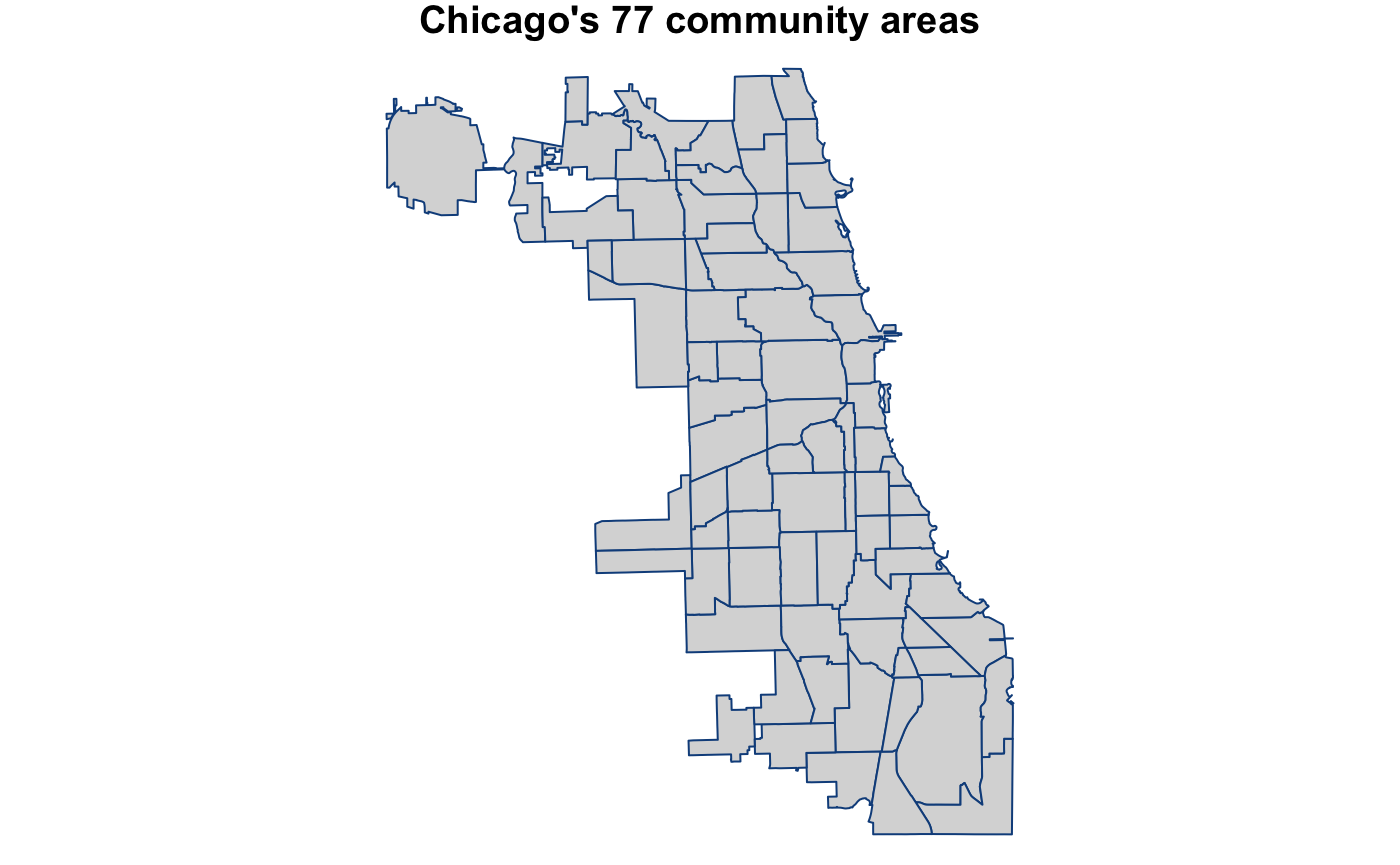
While the city boundary is helpful for generating city-wide statistics, researchers typically use the 77 Chicago community areas when creating local-level statistics.
pointdexter makes both polygons available as sf and SpatialPolygonsDataFrame objects.
# load city boundary data ----
data("city_boundary_spdf")

# load community area data ----
data("community_areas_spdf")

# visualize polygons -----
# note: clear plot space
par(mar = c(0, 0, 1, 0))

# plot city boundary
plot(city_boundary_spdf
     , main = "City of Chicago boundary"
     , col = "gray85"
     , border = "dodgerblue4")

# plot community areas
plot(community_areas_spdf
     , main = "Chicago's 77 community areas"
     , col = "gray85"
     , border = "dodgerblue4")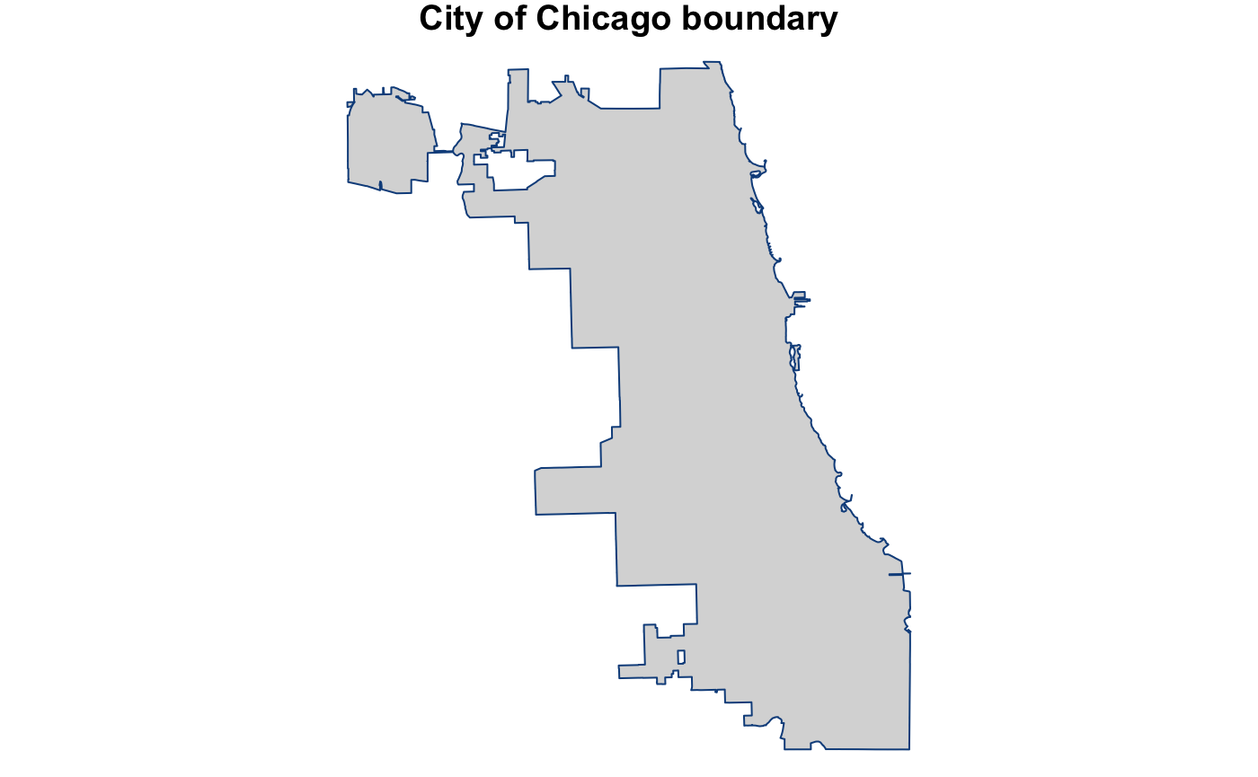
Step 1. Use GetPolygonBoundaries()
GetPolygonBoundaries() returns the longitudinal and latitudinal points that make up the boundary of the polygon(s). The first argument is the polygon stored in the sf or SpatialPolygonsDataFrame object.
One polygon
If my.polygon only contains one polygon, a matrix of coordinate pairs will be returned.
# create coordinate pair matrix for city of chicago boundary ----
boundary <-
  GetPolygonBoundaries(my.polygon = city_boundary_spdf)

# print first few records ----
kable(head(boundary)
        , caption = "Table 2. boundary is a matrix of coordinate pairs"
, col.names = c("long", "lat"))| long | lat |
|---|---|
| -87.93514 | 42.00089 |
| -87.93509 | 42.00094 |
| -87.93517 | 42.00333 |
| -87.93519 | 42.00430 |
| -87.93521 | 42.00491 |
| -87.93523 | 42.00573 |
Multiple polygons
Otherwise, a list of labeled matrices, with each matrix representing the coordinate pairs that make the boundary of each particular polygon in my.polygon.
# create list of coordinate pair matrices for each community area ----
community.area.boundaries <-
  GetPolygonBoundaries(my.polygon = community_areas_spdf
                       , labels = community_areas_spdf$community)

# print first few records for two communities ----
kable(lapply(community.area.boundaries[c("AUSTIN", "WEST ELSDON")]
             , FUN = head)
      , caption = "Table 3. Austin (left) and West Elsdon's (right) boundaries"
      , col.names = c("long", "lat"))
|
|
Step 2. Use LabelPointsWithinPolygons()
LabelPointsWithinPolygons() identifies which longitudinal and latitudinal points lie within the polygon boundaries created from GetPolygonBoundaries().
The first two arguments of LabelPointsWithinPolygons() are the longitude and latitude columns that create your coordinate pairs of interest. The final argument - polygon.boundaries is the object you created from GetPolygonBoundaries().
polygon.boundaries is a matrix
If polygon.boundaries is a coordinate pair matrix, a logical vector will be returned identifying those points which lie in the polygon.
# identify cps schools that lie in Chicago ----
cps_sy1819$in_chicago <-
  LabelPointsWithinPolygons(lng = cps_sy1819$school_longitude
                            , lat = cps_sy1819$school_latitude
                            , polygon.boundaries = boundary)

# show first few records ----
kable(head(cps_sy1819[, c(relevant.columns, "in_chicago")])
, caption = "Table 4. A logical vector is returned when polygon.boundaries is a matrix")| school_id | short_name | school_longitude | school_latitude | in_chicago |
|---|---|---|---|---|
| 609760 | CARVER MILITARY HS | -87.59062 | 41.65629 | TRUE |
| 609780 | MARINE LEADERSHIP AT AMES HS | -87.72174 | 41.91604 | TRUE |
| 610304 | PHOENIX MILITARY HS | -87.68696 | 41.87912 | TRUE |
| 610513 | AIR FORCE HS | -87.63276 | 41.82814 | TRUE |
| 610390 | RICKOVER MILITARY HS | -87.66579 | 41.98902 | TRUE |
| 609754 | CHICAGO MILITARY HS | -87.61922 | 41.83055 | TRUE |
polygon.boundaries is a list of matrices
Otherwise, a character vector will be returned identifying those points that lie in each polygon.
# identify the community that each cps school lies in ----
cps_sy1819$community <-
  LabelPointsWithinPolygons(lng = cps_sy1819$school_longitude
                            , lat = cps_sy1819$school_latitude
                            , polygon.boundaries = community.area.boundaries)

# show first few records ----
kable(head(cps_sy1819[, c(relevant.columns, "in_chicago", "community")])
, caption = "Table 5. A character vector is returned when polygon.boundaries is a list of labeled matrices")| school_id | short_name | school_longitude | school_latitude | in_chicago | community |
|---|---|---|---|---|---|
| 609760 | CARVER MILITARY HS | -87.59062 | 41.65629 | TRUE | RIVERDALE |
| 609780 | MARINE LEADERSHIP AT AMES HS | -87.72174 | 41.91604 | TRUE | LOGAN SQUARE |
| 610304 | PHOENIX MILITARY HS | -87.68696 | 41.87912 | TRUE | NEAR WEST SIDE |
| 610513 | AIR FORCE HS | -87.63276 | 41.82814 | TRUE | ARMOUR SQUARE |
| 610390 | RICKOVER MILITARY HS | -87.66579 | 41.98902 | TRUE | EDGEWATER |
| 609754 | CHICAGO MILITARY HS | -87.61922 | 41.83055 | TRUE | DOUGLAS |
Conclusion
pointdexter finds the boundaries of whatever polygon you give so that you can identify coordinate pairs that lie within it. This is useful when wanting to generate local statistics for particular communities.
# identify the school ratings for high schools in Austin ----

# filter cps schools
austin.hs <-
  cps_sy1819[cps_sy1819$community == "AUSTIN" & cps_sy1819$is_high_school, ]

# arrange data by overall rating
austin.hs <- austin.hs[order(austin.hs$overall_rating), ]

# show results
kable(austin.hs[, c(relevant.columns , "overall_rating",
              "is_high_school", "community")]
      , caption = "Table 6. Austin's highest rank high school is YCCS - Scholastic Academy, SY1819"
, row.names = FALSE)| school_id | short_name | school_longitude | school_latitude | overall_rating | is_high_school | community |
|---|---|---|---|---|---|---|
| 400123 | YCCS - SCHOLASTIC ACHIEVEMENT | -87.74254 | 41.88045 | Level 1+ | TRUE | AUSTIN |
| 400127 | YCCS - AUSTIN CAREER | -87.76022 | 41.89498 | Level 1 | TRUE | AUSTIN |
| 400144 | YCCS - WESTSIDE HOLISTIC | -87.74881 | 41.90224 | Level 1 | TRUE | AUSTIN |
| 610244 | CLARK HS | -87.75333 | 41.87288 | Level 2+ | TRUE | AUSTIN |
| 610245 | DOUGLASS HS | -87.76767 | 41.89037 | Level 2 | TRUE | AUSTIN |
| 610518 | AUSTIN CCA HS | -87.76192 | 41.88599 | Level 2 | TRUE | AUSTIN |
Session Info
## R version 3.5.2 (2018-12-20)
## Platform: x86_64-apple-darwin15.6.0 (64-bit)
## Running under: macOS High Sierra 10.13.6
##
## Matrix products: default
## BLAS: /Library/Frameworks/R.framework/Versions/3.5/Resources/lib/libRblas.0.dylib
## LAPACK: /Library/Frameworks/R.framework/Versions/3.5/Resources/lib/libRlapack.dylib
##
## locale:
## [1] en_US.UTF-8/en_US.UTF-8/en_US.UTF-8/C/en_US.UTF-8/en_US.UTF-8
##
## attached base packages:
## [1] stats     graphics  grDevices utils     datasets  methods   base
##
## other attached packages:
## [1] knitr_1.21        sp_1.3-1          pointdexter_0.1.0
##
## loaded via a namespace (and not attached):
##  [1] Rcpp_1.0.0       rstudioapi_0.9.0 xml2_1.2.0       magrittr_1.5
##  [5] roxygen2_6.1.1   units_0.6-2      MASS_7.3-51.1    lattice_0.20-38
##  [9] R6_2.3.0         rlang_0.3.1      highr_0.7        stringr_1.3.1
## [13] tools_3.5.2      grid_3.5.2       xfun_0.4         e1071_1.7-0
## [17] DBI_1.0.0        class_7.3-14     htmltools_0.3.6  commonmark_1.7
## [21] yaml_2.2.0       digest_0.6.18    assertthat_0.2.0 rprojroot_1.3-2
## [25] sf_0.7-2         pkgdown_1.3.0    crayon_1.3.4     splancs_2.01-40
## [29] fs_1.2.6         memoise_1.1.0    evaluate_0.12    rmarkdown_1.11
## [33] stringi_1.2.4    compiler_3.5.2   desc_1.2.0       backports_1.1.3
## [37] classInt_0.3-1