Make a Choropleth Map
Cristian E. Nuno
December 28, 2017
Introduction
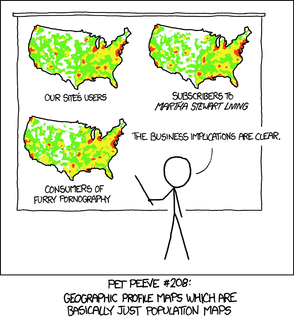 Image courtesy of XKCD
Choropleth maps are popular. But - as the comic above shows - their popularity requires map makers to take great care in the presentation of the data.
Choropleth Maps
At its core, choropleth maps rely on color to represent different scales of data. Rather than recreate definitions, please find the following resources as great places to dive into the background and commentary on choropleth maps:
Penn State’s GEOG 486: Geography and Visualization is a tremendous resource to enrich yourself as an amateur geographer. Click here for their take on choropleth maps.
When Maps Lie - written by Andrew Wiseman - brings in contempary example of overly ambitious maps.
How to Lie with Maps - written by Syracuse University’s Maxwell School of Citizenship and Public Affairs Distinguished Professor of Geography, Dr. Mark Monmonier - is the classic text on the misuse of maps.
Creating Maps in R - written by my former professor and current academic director of the M.S. in Program Evaluation at Arizona State University’s College of Public Services & Community Solutions, Dr. Jesse Lecy - provides a comprehensive overview on producing maps in R.
Import Necessary Packages
To follow the tutorial, you’ll need to install the following packages installed:
maptools: Tools for Reading and Handling Spatial Objects.sp: Classes and methods for spatial data.raster: Geographic Data Analysis and Modeling.rgdal: Primarily used to create spatial data frames, using the Geospatial Data Abstraction Library.
# install necessary packages
# install.packages( pkgs = c("maptools"
#                            , "sp"
#                            , "raster"
#                            , "rgdal"
#                            )
#                   )
# import packages into namespace
library( maptools )
library( sp )
library( raster )
library( rgdal )
Create Choropleth Map
Create Sample Data
This tutorial uses made up date that tallies the number of cool people per state for the year 2017.
# including D.C.
sample.data <- data.frame( State = append( x = datasets::state.abb
                                           , values = "DC"
                                           , after = 7
                                           )
                           , Count_Awesome_People = 1:51
                           , stringsAsFactors = FALSE
                           )
Define Colors
Ranging from dull to exciting, let’s create colors that will be used to define groups within the values of sample.data$Count_Awesome_People.
# make colors from gray to dodgerblue4
color.function <- colorRampPalette( c("#CCCCCC","#104E8B") )
# decide how many groups I want, in this case 5
color.ramp <- color.function( 5 )
Assign Colors to Groups
Assign each row in sample.data a color value, based on their sample.data$Count_Awesome_People value.
sample.data$color <-
  as.character(
    cut( # use cut to divide the range of Count_Awesome_People value into intervals
      x = rank( sample.data$Count_Awesome_People ) # used to rank the values (always assigning order)
      , breaks = 5 # define the numbers of groups to place certain values of Count_Awesome_People
      , labels = color.ramp # label the groups a color from color.ramp
    )
  )
Import U.S. Census Shapefiles
The United States Census Bureau contains geographic boundaries - otherwise known as cartographic boundary shapefiles - from everything to congressional districts to school districts.
This tutorial uses the U.S. state shapefiles from 2016 - with the lowest resolution to speed up downloading time. Since the shapefiles come in a .zip file, there are some extra steps needed prior to successfully importing them as one spatial data frame.
Using rgdal::readOGR()
Jeffrey Hollister’s Things I Forget: Reading a Shapefile in R with readOGR reminds all of us how to assemble a spatial data frame from the shapefiles within that .zip folder using two arguments within rgdal::readOGR():
dsn is the directory (without a trailing backslash) and the layer is the shapefile name without the .shp.
dsn stands for data source name that can either be a file name or a folder; layer is the name of the shapefile - as told by the extension (i.e. .json, .geojson, .shp). For more information on layer, please see OGR Vector Formats and OGR shapefile encoding.
# set working directory to store shape files
setwd( "/Users/cristiannuno/RStudio_All/US_State_Shapefiles" )

# save URL of U.S. census state boundary shape files
shapefile.url <- "http://www2.census.gov/geo/tiger/GENZ2016/shp/cb_2016_us_state_20m.zip"

# download the file into working directory and be sure to name the zip file
download.file( url = shapefile.url
               , destfile = "2016_US_State_Shapefile.zip"
               )
# unzip the zip file
unzip( zipfile = "2016_US_State_Shapefile.zip" )

# transform to spatial data frame
# https://www.r-bloggers.com/things-i-forget-reading-a-shapefile-in-r-with-readogr/
us.states <- readOGR( dsn = getwd()
                      , layer = "cb_2016_us_state_20m"
                      , stringsAsFactors = FALSE
                      )
Extracting, Resizing, and Relocating Alaska & Hawaii
R-blogger’s user Bob Rudis (hrbmstr)’s article - Moving The Earth (well, Alaska & Hawaii) With R - does the best job explaining how to reposition these two states just below the Southwest portion of the U.S:
- extract them from the main shapefile data frame
- perform rotation, scaling and transposing on them
- ensure they have the right projection set
- merge them back into the original spatial data frame
In the article, he goes onto show he performed this task using R. None of this portion of the code is mine; it is all Bob’s work. Thank you Bob Rudis for sharing your knowledge! You can learn more from Bob by seeing his latest work on GitHub.
# convert it to Albers equal area
# specify the project arguments
us.states <- spTransform( x = us.states
                          , CRSobj = CRS("+proj=laea +lat_0=45 +lon_0=-100 +x_0=0 +y_0=0 +a=6370997 +b=6370997 +units=m +no_defs")
                          )
# extract, then rotate, shrink & move alaska (and reset projection)
# need to use state IDs via
# # https://www.census.gov/geo/reference/ansi_statetables.html

# extract alaska
alaska <- us.states[ which( us.states$STATEFP == "02" ) , ]

# rotate Alaska, 50 degrees counter clock wise
alaska <- elide( obj = alaska
                 , rotate = -50
                 )
# shrink Alaska
alaska <- elide( obj = alaska
                 , scale = max( apply( X = bbox( alaska )
                                       , MARGIN = 1
                                       , FUN = diff
                                       )
                                ) / 2.3
                 )
# now shift alaska's coordinates
alaska <- elide( obj = alaska
                 , shift = c( -2100000, -2500000 )
                 )
# reset projects, as in now that it's modified
# place the modified version onto the us.states spatial df
proj4string( alaska ) <- proj4string( us.states )

# extract, then rotate & shift hawaii
hawaii <- us.states[ which( us.states$STATEFP=="15" ) , ]
hawaii <- elide(obj = hawaii
                , rotate = -35
                )
hawaii <- elide(obj = hawaii
                , shift = c( 5400000, -1400000 )
                )
proj4string( hawaii ) <- proj4string( us.states )

# remove old states and put new ones back in; note the different order
# we're also removing puerto rico in this example but you can move it
# between texas and florida via similar methods to the ones we just used
us.states <- us.states[ which( !us.states$STATEFP %in% c("02", "15", "72") ) , ]
us.states <- rbind(us.states, alaska, hawaii)
Use sp::merge() to Merge Non-Spatial Data onto the Spatial Data
To keep the spatial attributes intact, while joining the columns from non-spatial data, the sp::merge() function is best for the job.
us.states <- sp::merge( x = us.states
                        , y = sample.data
                        , by.x = "STUSPS"
                        , by.y = "State"
                        )
Plot
After all that hard work, now is the time to create the choropleth map.

# clear margin space and set plot background color
par( mar = c(2, 0, 3, 0 )
     , bg = "ghostwhite"
     )

# plot the U.S.
# fill each state with its color value
# color the borders a light gray
plot( x = us.states
      , col = us.states$color
      , border = "gray70"
      )
# add main title
mtext( side = 3
       , adj = 0.05
       , line = 1.8
       , cex = 1.2
       , text = "Awesome People by State, 2017"
       )
# add sub title
mtext( side = 3
       , adj = 0.075
       , line = 1
       , cex = 0.75
       , text = "Choropleth maps rely on color to represent different groups in categorical data."
       )
# add data source
mtext( side = 1
       , adj = 0.95
       , line = 0.5
       , cex = 0.75
       , text = "Source: My imagination."
       )
# Find the center of each region
# and label each state with its abbreviated name
raster::text( x = us.states[ which( !us.states$STUSPS %in% "DC" ) , ]
              , labels = us.states$STUSPS[ which( !us.states$STUSPS %in% "DC" ) ]
              , halo = TRUE
              , hc = "black"
              , hw = 0.1
              , col = "white"
              , cex = 0.55
)
# add legend
# text determined from:
# levels( cut( x = us.states$Count_Awesome_People, breaks = 5))
# note: the output must be read in interval notation
# http://www.mathwords.com/i/interval_notation.htm
legend( x = "right"
        , legend = c(  "42 - 51"
                     , "32 - 41"
                     , "22 - 31"
                     , "12 - 21"
                     , "  1 - 11"
                     )
        , pt.cex = 2
        , pch = 15
        , col = rev( x = color.ramp )
        , cex = 1
        , bty = "n"
        )
About Me
Thank you for reading this tutorial. My name is Cristian E. Nuno and I am an aspiring data scientist. To see more of my work, please visit my professional portfolio Urban Data Science.
Session Info
# Print version information about R, the OS and attached or loaded packages.
sessionInfo()
R version 3.4.3 (2017-11-30) Platform: x86_64-apple-darwin15.6.0 (64-bit) Running under: macOS Sierra 10.12.6
Matrix products: default BLAS: /System/Library/Frameworks/Accelerate.framework/Versions/A/Frameworks/vecLib.framework/Versions/A/libBLAS.dylib LAPACK: /Library/Frameworks/R.framework/Versions/3.4/Resources/lib/libRlapack.dylib
locale: [1] en_US.UTF-8/en_US.UTF-8/en_US.UTF-8/C/en_US.UTF-8/en_US.UTF-8
attached base packages: [1] stats graphics grDevices utils datasets methods base
other attached packages: [1] raster_2.6-7 rgdal_1.2-16 maptools_0.9-2 sp_1.2-5
loaded via a namespace (and not attached): [1] Rcpp_0.12.14 lattice_0.20-35 digest_0.6.13 rprojroot_1.3-1 [5] grid_3.4.3 backports_1.1.2 magrittr_1.5 evaluate_0.10.1 [9] stringi_1.1.6 rmarkdown_1.8 tools_3.4.3 foreign_0.8-69 [13] stringr_1.2.0 yaml_2.1.16 rsconnect_0.8.5 compiler_3.4.3 [17] htmltools_0.3.6 knitr_1.17
Copyright © 2017 - 2018. Urban Data Science. All rights reserved. See Disclaimer for further details.